The Fortran Language

Fortran was the first high-level language and was developed in the fifties. The languages has since the developed through a number of standards Fortran IV (1966), Fortran 77, Fortran 90, Fortran 95, Fortran 2003, Fortran 2008 and the latest Fortran 2018. The advantages with standardised languages is that the code can be run on different computer architectures without modification. In every new standard the language has been extended with more modern language elements. To be compatible with previous standards older language elements are not removed. However, language elements that are considered bad or outdated can be removed after 2 standard revisions. As an example Fortran 90 is fully backwards compatible with Fortran 77, but in Fortran 95 some older language constructs where removed.

The following sections gives a short introduction to the modern Fortran language from Fortran 90 and above. The description is centered on the most important language features. A more thorough description of the language can be found in the book Modern Fortran Explained [metcalfreid18].

Program structure

Every Fortran-program must have a main program routine. From the main routine, other subroutines that make up the program are called. The syntax for a main program is:

program [program-name]
[specification statements]
[executable statements]
[contains]
[subroutines]
end [program [program-name]]

From the syntax it can be seen that the only identifier that must be included in main program definition is end.

The syntax for a subroutine and functions are defined in the same way, but the program identifier is replaced with subroutine or function. A proper way of organizing subroutines is to place these in separat files or place the in modules (covered in upcoming sections). Subroutines can also be placed in the main program contains-section, which is the preferred method if all subroutines are placed in the same source file. The code below shows a simple example of a main program with a subroutine in Fortran.

program sample1

    integer, parameter :: dp=selected_real_kind(15,300)
    real(kind=dp) :: x, y
    real(kind=dp) :: k(20,20)

    x = 6.0_dp
    y = 0.25_dp

    write(*,*) x
    write(*,*) y
    write(*,*) dp

    call myproc(k)

    write(*,*) k(1,1)

contains

subroutine myproc(k)
	
    integer, parameter :: dp=selected_real_kind(15,300)
    real(kind=dp) :: k(20,20)

    k=0.0_dp
    k(1,1) = 42.0_dp

    return

end subroutine myproc

end program sample1

The program source code can contain upper and lower case letters, numbers and special characters. However, it should be noted that Fortran does not differentiate between upper and lower case letters. The program source is written starting from the first position with one statement on each line. If a row is terminated with the charachter &, this indicates that the statement is continued on the the next line. All text placed after the character ! is a comment and wont affect the function of the program. Even if the comments don’t have any function in the program they are important for source code readability. This is especially important for future modification of the program. In addition to the source code form described above there is also the possibility of writing code in fixed form, as in Fortran 77 and earlier versions. In previous version of the Fortran standard this was the only source code form available.

Variables

Variables are named references to data stored in memory. When specifying variables in Fortran, the data type of the data must also be specified. This means that Fortran is a strongly typed language compared to Python where data types of variables can change during code execution. Python is a dynamically typed language.

By default Fortran assumes that variables starting with letters I to N are assumed to be integers all other variables are assumed to be floating point variables (real). This is also called the implict type rule and is considered bad practice in Fortran, but is default because many Fortran programs are still relying on this rule. Modern Fortran application should always disable the implict type rule by adding the following statement in each code unit:

implicit none

This is also described in more detail in the following sections.

Naming of variables

Variables in modern Fortran consists of 1 to 31 alphanumeric characters (letters except and , underscore and numbers). The first character of a variable name must be a letter. Allowable variable names can be:

a
a_thing
x1
mass
q123
time_of_flight

Variable names can consist of both upper case and lower case letters. It should be noted that a and A references the same variable. Invalid variables names can be:

1a      ! First character not a letter
a thing ! Contains a space character
%       ! Contains a non-alphanumeric character

Data types and declarations

There are 5 built-in data types in Fortran:

• integer, Integers.

• real, Floating point numbers.

• complex, Complex numbers.

• logical, Boolean values.

• character, Strings and characters.

The syntax for a variable declaration is:

type [[,attribute]... ::] entity-list

type defines the variable type and can be integer, real, complex, logical, **character or type( type-name ). attribute defines additional special attributes or how the variable is to be used. The following examples shows some typical Fortran variable declarations.

integer :: a     ! Scalar integer variable
real    :: b     ! Scalar floating point variable
logical :: flag  ! boolean variable

real :: D(10)    ! Floating point array consisting of 10 elements
real :: K(20,20) ! Floating point array of 20x20 elements

integer, dimension(10) :: C     ! Integer array of 10 elements

character :: ch                 ! Character
character, dimension(60) :: chv ! Array of characters
character(len=80) :: line       ! Character string
character(len=80) :: lines(60)  ! Array of strings

Constants are declared by specifying an additional attribute, parameter. A declared constant can be used in following variable declarations. An example of use is shown in the following example.

integer, parameter :: A = 5 ! Integer constant
real :: C(A)                ! Floating point array where
                            ! the number of elements is
                            ! specified by A

The precision and size of the variable type can be specified by adding a parenthesis directly after the type declaration. The variables A and B in the following example are declared as floating point scalars with different precisions. The number in the parenthesis denotes for many architectures, how many bytes a floating point variable is represented with. This is however not standardised and should not be relied upon.

real(8) :: A
real(4) :: B
integer(4) :: I

To be able to choose the correct precision for a floating point variable, Fortran has a built in function selected_real_kind that returns the value to be used in the declaration with a given precision. This is illustrated in the following example.

integer, parameter :: dp = selected_real_kind(15,300)
real(kind=dp) :: X,Y

In this example the floating point variable should have at least 15 significant decimals and could represent numbers from \(10^{-300}\) to \(10^{300}\). For several common architectures selected_real_kind will return the value 8. The advantage of using the above approach is that the precision of the floating point values can be specified in a architectural independent way. The precision constant can also be used when specifying numbers in variable assignments as the following example illustrate.

X = 6.0_dp

The importance of specifying the precision for assigning scalar values to variables is illustrated in the following example.

program constants

    implicit none

    integer, parameter :: dp = selected_real_kind(15,300)

    real(dp) :: pi1, pi2
    pi1 = 3.141592653589793
    pi2 = 3.141592653589793_dp

    write(*,*) 'pi1 = ', pi1
    write(*,*) 'pi2 = ', pi2

    stop

end program constants

The program gives the following results:

pi1 = 3.14159274101257
pi2 = 3.14159265358979

Run example

The scalar number assigned to the variable pi1 is chosen by the compiler to be represented by the least number of bytes floating point precision, in this case real(4), which is shown in the output from the above program.

Variable declarations in Fortran always precedes the executable statements in the main program or in a subroutine. Declarations can also be placed directly after the module identifier in modules.

Implicit type rule

Variable do not have to be declared in Fortran. The default is that variables starting I, J,…, N are defined as integer and variables starting with A, B,… ,H or O, P,… , Z are defined as real. This kind of implicit variable declaration is not recommended as it can lead to programming errors when variables are misspelled. To avoid implicit variable declarations the following declaration can be placed first in a program or module:

implicit none

This statement forces the compiler to make sure that all variables are declared. If a variable is not declared the compilation is stopped with an error message. This is default for many other strongly typed languages such as, C, C++ and Java.

Assignment of variables

The syntax for scalar variable assignment is,

variable = expr

where variable denotes the variable to be assigned and expr the expression to be assigned. The following example assign the a variable the value 5.0 with the precision defined in the constant ap.

a = 5.0_dp

Assignment of boolean variables are done in the same way using the keywords, .false. and .true. indicating a true or false value. A boolean expression can also be used int the assignment. In the following example the variable, flag, is assigned the value .false..

flag =.false.

Assignment of strings are illustrated in the following example.

character(40) :: first_name
character(40) :: last_name
character(20) :: company_name1
character(20) :: company_name2

...

first_name = 'Jan'
last_name = "Johansson"
company_name1 = "McDonald's"
company_name2 = 'McDonald''s'

The first variable, first_name, is assigned the text ‘’Jan’’, remaining characters in the string will be padded with spaces. A string is assigned using citation marks, ‘’ or apostrophes, ‘. This can be of help when apostrophes or citation marks is used in strings as shown in the assignemnt of the variables, company_name1 och company_name2.

Defined and undefined variables

A variable in Fortran that has been assigned a value is considered to be defined and can be used safely. Variables that are not assigned values are said to be undefined and should not be used.

A program containing undefined variables will not fail compilation. Memory for undefined variables will be reserved and can be referenced. However, values of undefined variables are not automatically set to zero and references memory locations with unknown values. Often these variables will return garbage or random values. As rule always initialise variables to a default values or make sure they are assigned a value from another variable reference.

The following example shows an example of referencing defined and undefined variables.

program undef1

    implicit none

    integer, parameter :: dp = selected_real_kind(15,300)

    real(dp) :: a, b
    character(40) :: s1, s2

    a = 42.0_dp ! --- Defined
    s1 = 'My defined string'

    print*, a
    print*, b
    print*, s1
    print*, s2

end program undef1

This will print the following:

  42.000000000000000
  8.2890460584580950E-317
My defined string

Run example

The reason for the 8.28…E-317 value is that the variable reference b points to its given memory location, but no value has been assigned to this location and will contain whatever was in memory when the program was executed. Fortran will interpret the values at this location as a floating point value and present it as such. This illustrates why it is a good idea to initialise variables to 0.0_dp or make sure they will be assigned values from other variable references.

Derived datatypes

In certain cases it can be beneficial to create your own data types to handle the behavior of your program. To create new data types in Fortran you can create derived data types using the type-statement. Using this statement a new data type can be created by grouping existing Fortran data types into a new type. In the following example a data type of a particle is defined:

type particle
    real(dp) :: x
    real(dp) :: y
    real(dp) :: z
    real(dp) :: m
end type particle

The new data type can now be used like any other data type in Fortran. To create a variable reference to a derived data type the type keyword precedes the name of the data type in the declaration. As in the following example:

type(particle) :: p0

The members of the derived data types are accessed using the %-operator. In the following example the members of the variable p0 are assigned values:

p0 % x = 0.0_dp
p0 % y = 0.0_dp
p0 % z = 0.0_dp
p0 % m = 1.0_dp

Derived data types can contain multiple Fortran data types:

type particle
    real(dp)  :: x
    real(dp)  :: y
    real(dp)  :: z
    real(dp)  :: m
    logical   :: active
    integer   :: id
    character :: name(8)
end type particle

Operators and expressions

The following arithmetic operators are defined in Fortran:

Operator	Description
**	power to
*	multiplication
/	division
+	addition
-	subtraction

Parenthesis are used to specify the order of different operators. If no parenthesis are given in an expression operators are evaluated in the following order:

1. Operations with **

2. Operations with * or /

3. Operations with + or –

The following code illustrates operator precedence.

c = a+b/2 ! is equivalent to :math:`a+(b/2)`
c = (a+b)/2 ! in this case :math:`(a+b)` is evaluated and then :math:`/` 2

Relational operators:

Operator	Description
< or .lt.	less than
<= or .le.	less than or equal to
> or .gt.	greater than
>= or .ge.	greater than or equal to
== or .eq.	equal to
/= or .ne.	not equal to

Logical operators:

Operator	Description
.and.	and
.or.	or
.not.	not

Numeric expressions

Numeric expressions in Fortran consist of operands of the built-in data types integer, fkeyw{real} or complex.

If the operands only consists of integer it is important to note that integer divisions are rounded towards 0. The following example illustrates this:

program expr1

    print*, 6/3
    print*, 8/3   ! 2.6666... rounded down to 2
    print*, -8/3  ! -2.666... rounded up to 2

end program expr1

Running the program will result in the following output:

2
2
-2

There are also some other things to be careful with when working with integer expressions. Consider the following example:

program expr2

    print*, 2**3
    print*, 2**(-3)

end program expr2

When run will give the following output:

8
0

The reason for the 0 in the second expression is that 2**(-3) is the same as 1/2**3, which will be truncated to 0 as an integer expression.

When mixing data types in expressions, weaker data types will be converted to the stronger type. The result of the expression will be of the stronger type. real is stronger than integer. Consider the following code:

real(dp) :: a
integer :: i
real(dp) :: b

b = a * i

Here, the i variable reference will be converted to real(dp) when the expression is evaluated.

Arrays and matrices

In scientific and technical applications matrices and arrays are important concepts. As Fortran is a language mainly for technical computing, arrays and matrices play a vital role in the language.

Declaring arrays and matrices can be done in two ways. In the first method the dimensions are specified using the special attribute, dimension, after the data type declaration. The second method, the dimensions are specified by adding the dimensions directly after the variable name. The following code illustrate these methods of declaring arrays.

integer, parameter :: dp = selected_real_kind(15,300)
real(dp), dimension(20,20) :: K ! Matrix 20x20 elements
real(dp) :: fe(6) ! Array with 6 elements

The default starting index in arrays is 1. It is however possible to define custom indices in the declaration, as the following example shows.

real(ap) :: idx(-3:3)

This declares an array, idx with the indices [-3, -2, -1, 0, 1, 2, 3], which contains 7 elements.

Array assignment

Arrays are assigned values either by explicit indices or the entire array in a single statement. The following code assigned the variable, K, the value 5.0 at position row 5 and column 6.

K(5,6) = 5.0_dp

If the assignment had been written as

K = 5.0_dp

the entire array, K, would have been assigned the value 5.0. This is an efficient way of assigning entire arrays initial values.

Explicit values can be assigned to arrays in a single statement using the following assignment.

real(dp) :: v(5) ! Array with 5 elements
v = (/ 1.0_dp, 2.0_dp, 3.0_dp, 4.0_dp, 5.0_dp /)

This is equivalent to an assignment using the following statements.

v(1) = 1.0_dp
v(2) = 2.0_dp
v(3) = 3.0_dp
v(4) = 4.0_dp
v(5) = 5.0_dp

The number of elements in the list must be the same as the number of elements in the array variable.

Assignments to specific parts of arrays can be achieved by slicing. The following example illustrates this concept.

program slicing

    implicit none
    real :: A(4,4)
    real :: B(4)
    real :: C(4)

    B = A(2,:) ! Assigns B the values of row 2 in A
    C = A(:,1) ! Assigns C the values of column 1 in A

    stop

end program slicing

Using slicing rows or columns can be assigned in single statements as shown in the following code:

! Assign row 5 in matrix K the values 1, 2, 3, 4, 5

K(5,:) = (/ 1.0_dp, 2.0_dp, 3.0_dp, 4.0_dp, 5.0_dp /)

! Assign the array v the values 5, 4, 3, 2, 1

v = (/ 5.0_dp, 4.0_dp, 3.0_dp, 2.0_dp, 1.0_dp /)

Array expressions

In modern Fortran expressions can also be used on arrays. The operators will then apply element wise to the in the expression. For this to work the arrays must be of the same size. Array expression can also contain scalar values. These will be broadcast to the array elements. Consider the following arrays:

real :: a(10,20), b(10,20), c(10,20)
real :: u(5), v(5)

The following expression will divide all values in a with the values in b.

c = a/b

This is equivalent to:

do i=1,10
    do j=1,20
        c(i,j) = a(i,j)/b(i,j)
    end do
end do

It is important to make sure the resulting variable on the left side of the assignment has the same size as the resulting array expression.

The following expression adds a scalar value to all elements in the array v:

u = v + 1.0

This is equivalent to:

do i=1,5
    u(i) = v(i) + 1.0
end do

It is also possible to use slicing to extract a ‘’slice’’ that can be used in an array expression:

u = 5.0/v + a(1:5,5)

Which is equivalent to:

do i=1,5
    u(i) = 5.0/v(i) + a(i,5)
end do

Array storage

Memory allocation by the operating system is done in linear blocks of bytes. The operating system does not have the concept of multidimensional arrays. This is a concept introduced by the programming language, in this case Fortran, to make it easier for us to implement algorithms and access values stored in memory.

There are 2 conventions of storing 2D arrays in memory, by column and by row. Fortran as a convention stores arrays by column and C by row. The following figure illustrates this concept:

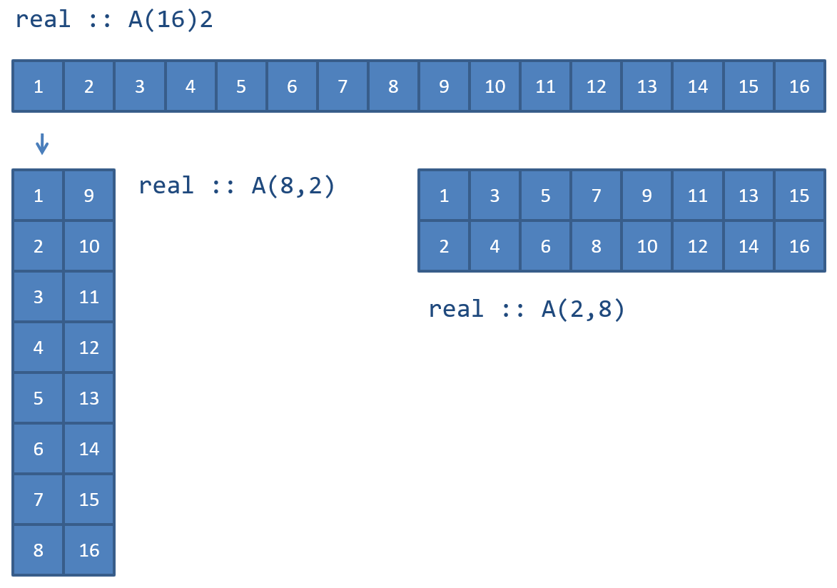
Fig. 1 Arrays in memory.

The storage of arrays in memory is especially important when calling libraries implemented in other languages, which usually stores arrays by row. The Python library NumPy by default stores all arrays using the C convention. Calling a Fortran subroutine with a pointer to these arrays will probably result in undefined behavior. NumPy supports column ordered arrays by supplying the array-constructor with the option pkeyw{order=F}.

Allocatable arrays

In Fortran 77 and earlier versions of the standard it was not possible to dynamically allocate memory during program execution. This capability is now available in Fortran 90 and later versions. To declare an array as dynamically allocatable, the attribute allocatable must be added to the array declaration. The dimensions are also replaced with a colon, :, indicating the number of dimensions in the declared variable. A typical allocatable array declaration is shown in the following example.

real, dimension(:,:), allocatable :: K

In this example the two-dimensional array, K, is defined as allocatable. To indicate that the array is two-dimensional is done by specifying dimension(:,:) in the variable attribute. To declare a one-dimensional array the code becomes:

real, dimension(:), allocatable :: f

Variables with the allocatable attribute can’t be used until memory is allocated. Memory allocation is done using the allocate method. To allocate the variables, K,f, in the previous examples the following code is used.

allocate(K(20,20))
allocate(f(20))

When the allocated memory is no longer needed it can be deallocated using the command, deallocate, as the following code illustrates.

deallocate(K)
deallocate(f)

An important issue when using dynamically allocatable variable is to make sure the application does not ‘’leak’’. ‘’Leaking’’ is term used by applications that allocate memory during the execution and never deallocate used memory. If unchecked the application will use more and more resources and will eventually make the operating system start swapping and perhaps become also become unstable. A rule of thumb is that an allocate statement should always have corresponding deallocate.

Array subobjects

In many situations you want to work on smaller parts or slices of existing arrays. In Modern Fortran this can be accomplished by using the subobject feature. We will illustrate the concept of subobjects by an example. Consider the following declarations of an 2D- and 1D array:

use utils

real(dp) :: A(10,10)
real(dp) :: v(10)

To make sure we don’t have any junk values in the arrays, we initialise these with random values between 1 and 0.

call init_rand()
call set_print_format(10, 4, 'F')

call rand_mat(A, 0.0_dp, 1.0_dp)
call rand_vec(v, 0.0_dp, 1.0_dp)

We print the arrays, so that we can see the structure:

call print_matrix(A, 'a')
print*, loc(A)

call print_vector(v, 'c')
print*, loc(v)

The print-statements are added to show the actual memory address, so we can see what happens when we create subobjects.

Matrix a ( 10 x  10) DP
---------------------------------------------------------------------- ...
    0.7112    0.6538    0.9200    0.7415    0.7460    0.4596    0.9778 ... 0.4111    0.0399    0.7354    0.9505    0.4428    0.7871    0.7390 ...
    0.9814    0.4057    0.4292    0.3406    0.6673    0.2120    0.9523 ...
    0.1369    0.5396    0.4405    0.7577    0.9942    0.7274    0.2653 ...
    0.7179    0.9883    0.5549    0.6374    0.1337    0.9464    0.7786 ...
    0.2915    0.8634    0.3962    0.8088    0.5708    0.9827    0.8841 ...
    0.8294    0.8191    0.5452    0.2079    0.1126    0.8199    0.2020 ...
    0.0706    0.6945    0.7744    0.3474    0.2566    0.6155    0.0921 ...
    0.3754    0.7855    0.9828    0.3965    0.9551    0.2119    0.2718 ...
    0.4026    0.5287    0.6198    0.9967    0.5866    0.6598    0.4024 ...
---------------------------------------------------------------------- ...
    140722079206560

Vector c ( 10) DP
---------------------------------------------------------------------- ...
    0.9092    0.4976    0.6361    0.0355    0.7865    0.2197    0.8824 ...
---------------------------------------------------------------------- ...
    140722079206480

In the first example we are extracing the first column of the A array:

call print_vector(A(:,1))
print*, loc(A(:,1))

This will give us the following output:

Vector ( 10)
---------------------------------------------------------------------- ...
    0.7112    0.4111    0.9814    0.1369    0.7179    0.2915    0.8294 ...
---------------------------------------------------------------------- ...
    140722079206560

From the output we can see that i seems to be the first column of the A array. We can also see that the memory location of the subobject is equivalent to the memory location of the A-array. This is due to the fact that memory for the A-array is stored column wise access a slice in this direction can be done directly without copying.

If we instead extract the first row of the A-array:

call print_vector(A(1,:))
print*, loc(A(1,:))

We get the following output:

Vector ( 10)
---------------------------------------------------------------------- ...
    0.7112    0.6538    0.9200    0.7415    0.7460    0.4596    0.9778 ...
---------------------------------------------------------------------- ...
            10278912

Here we can see that the memory location is in a completely different location. This is due to the fact that the compiler needs to make a temporary copy to create this slice. This is important to think about especially if working with large array slices that are passed in subroutine calls. This can lead to crashes as these slices often are allocated on the stack.

Below illustrates some other examples of using array sub objects:

call print_matrix(A(1:2,1:2))

call print_matrix(A(1:6:2,1:6:2))
print*, loc(A(1:6:2,1:6:2))

call print_matrix(A(:,1:2))
print*, loc(A(:,1:2))

This gives the following output:

Matrix (  2 x   2) DP
--------------------
    0.1233    0.2606
    0.8357    0.4479
--------------------
            27678720

Matrix (  3 x   3) DP
------------------------------
    0.1233    0.7812    0.1668
    0.4284    0.3687    0.6542
    0.2531    0.3314    0.3557
------------------------------
            27689200

Matrix ( 10 x   2) DP
--------------------
    0.1233    0.2606
    0.8357    0.4479
    0.4284    0.2254
    0.3541    0.3400
    0.2531    0.6490
    0.6420    0.5396
    0.5006    0.5849
    0.7185    0.3138
    0.8209    0.6203
    0.0232    0.9131
--------------------
    140728814257696

Conditional statements

One of the more important concepts in a programming language is the ability to execute code depending on certain conditions are fulfilled. Modern Fortran support this through the if- and the select-statement, which are described in this section.

The simplest form of if-statements in Fortran have the following syntax

if (scalar-logical-expr) then
    block
end if

where scalar-logical-expr is a boolean expression, that has to be evaluated as true, (.true.), for the statements in, block, to be executed. An extended version of the if-statement adds a else-block with the following syntax

if (scalar-logical-expr) then
    block1
else
    block2
end if

In this form the block1 will be executed if scalar-logical-expr is evaluated as true, otherwise block2 will be executed. A third form of if-statement contains one or more else if-statements with the following syntax:

if (scalar-logical-expr1) then
    block1
else if (scalar-logical-expr2) then
    block2
else
    block3
end if

In this form the scalar-logical-expr1 is evaluated first. If this expression is true block1 is executed, otherwise if scalar-logical-expr2 evaluates as true block2 is executed. If no other expressions are evaluated to true, block3 is executed. An if-statement can contain several else if-blocks. The use of if-statements is illustrated in the following example:

program logic

    implicit none

    integer :: x
    logical :: flag

    ! Read an integer from standard input

    write(*,*) 'Enter an integer value.'
    read(*,*) x

    ! Correct value to the interval 0-1000

    flag = .FALSE.

    if (x>1000) then
        x = 1000
        flag = .TRUE.
    end if

    if (x<0) then
        x = 0
        flag = .TRUE.
    end if

    ! If flag is .TRUE. the input value
    ! has been corrected.

    if (flag) then
        write(*,'(a,I4)') 'Corrected value = ', x
    else
        write(*,'(a,I4)') 'Value = ', x
    end if

    stop

end program logic

Another conditional construct is the case-statement.

select case (expression)
    case selector
        block
end select

In this statement the expression, expression is evaluated and the case-block with the corresponding selector is executed. To handle the case when no case-block corresponds to the expr, a case-block with the default keyword can be added. The syntax then becomes:

select case (expr)
    case selector
        block
    case default
        block
end select

Example of case-statement use is shown in the following example:

select case (display_mode)
    case (displacements)
        ...
    case (geometry)
        ...
end select

To handle the case when display_mode does not correspone to any of the alternatives the above code is modified to the following code.

select case (display_mode) case (displacements)
        ...
    case (geometry)
        ...
    case default
        ...
end select

The following program example illustrate how case-statements can be used.

program case_sample

    integer :: value

    write(*,*) 'Enter a value'
    read(*,*) value

    select case (value)
        case (:0)
            write(*,*) 'Less than one.'
        case (1)
            write(*,*) 'Number one!'
        case (2:9)
            write(*,*) 'Between 2 and 9.'
        case (10)
            write(*,*) 'Number 10!'
        case (11:41)
            write(*,*) 'Less than 42 but greater than 10.'
        case (42)
            write(*,*) 'Meaning of life or perhaps 6*7.'
        case (43:)
            write(*,*) 'Greater than 42.'
        case default
            write(*,*) 'This should never happen!'
    end select

    stop

end program case_sample

Run example

Repetitive statements

The most common repetitive statement in Fortran is the do-statement. The syntax is:

do variable = expr1, expr2 [,expr3]
    block
end do

variable is the control-variable of the loop. expr1 is the starting value, expr2 is the end value and expr3 is the step interval. If the step interval is not given it is assumed to be 1. There are two ways of controlling the execution flow in a do-statement. The exit command terminates the loop and program execution is continued after the do-statement. The cycle command terminates the execution of the current block and continues execution with the next value of the control variable. The example below illustrates the use of a do-statement.

program loop_sample

    implicit none

    integer :: i

    do i=1,20
        if (i>10) then
            write(*,*) 'Terminates do-statement.'
            exit
        else if (i<5) then
            write(*,*) 'Cycling to next value.'
            cycle
        end if
        write(*,*) i
    end do

    stop

end program loop_sample

The above program gives the following output:

Cycling to next value.
Cycling to next value.
Cycling to next value.
Cycling to next value.
5
6
7
8
9
10
Terminates do-statement.

Another repetitive statement available is the do while-statement. With this statement, the code block can execute until a certain condition is fulfilled. The syntax is:

do while (scalar-logical-expr)
    block
end do

The following code shows a simple do while-statement printing the function \(f(x)=sin(x)\).

x = 0.0
do while x<1.05
    f = sin(x)
    x = x + 0.1
    write(*,*) x, f
end do

There are other repetitive statements such as forall and where covered int the array features sections.

Built-in functions

Fortran has a number of built-in functions covering a number of different areas. The following tables list a selection of these. For a more thorough description of the built-in function please see, Metcalf and Reid [metcalfreid18].

Mathematical functions

Function	Description
acos(x)	Returns \(\arccos(x)\)
asin(x)	Returns \(\arcsin(x)\)
atan(x)	Returns \(\arctan(x)\)
atan2(y,x)	Returns \(\arctan(\frac{y}{x})\) from \(-\pi\) till math:-pi
cos(x)	Returns \(\cos(x)\)
cosh(x)	Returns \(\cosh(x)\)
exp(x)	Returns \(e^{x}\)
log(x)	Returns \(\ln(x)\)
log10(x)	Returns \(\lg(x)\)
sin(x)	Returns \(\sin(x)\)
sinh(x)	Returns \(\sinh(x)\)
sqrt(x)	Returns \(\sqrt{x}\)
tan(x)	Returns \(\tan(x)\)
tanh(x)	Returns \(\tanh(x)\)

Miscellaneous conversion functions

Function	Description
abs(a)	Returns absolute value of a
aint(a)	Truncates a floating point value
int(a)	Converts a floating point value to an integer
nint(a)	Rounds a floating point value to the nearest integer
real(a)	Converts an integer to a floating point value
max(a1,a2[,a3,…])	Returns the maximum value of two or more values
min(a1,a2[,a3,…])	Returns the minimum value of two or more values

Vector and matrix functions

Function	Description
dot_product(u, v)	Returns the scalar product of \(u\cdot v\)
matmul(A, B)	Matrix multiplication. The result must have the same for as \(\mathbf{AB}\)
transpose(C)	Returns the transpose \(\mathbf{C}^{T}\). Elementet \(C^{T}_{ij}\) motsvarar \(C_{ji}\)

Array functions

Function	Description
all(mask)	Returns true of all elements in the logical array mask are true. For example all(A>0)! returns true if all elements in \(\mathbf{A}\) are greater than 0.
any(mask)	Returns true if any of the elements in mask are true.
count(mask)	Returns the number of elements in mask that are true.
maxval(array)	Returns the maximum value of the elements in the array array.
minval(array)	Returns the minimum value of the elements in the array array.
product(array)	Returns the product of the elements in the array array.
sum(array)!	Returns the sum of elements in the array array.

Most built-in functions and operators in Fortran support arrays. The following example shows how functions and operators support operations on arrays.

real, dimension(20,20) :: A, B, C

C = A/B ! Division :math:`C_{ij}=A_{ij}/B_{ij}`

C = sqrt(A) ! Square root :math:`C_{ij}=\sqrt{A_{ij}}`

The following example shows how a stiffness matrix for a bar element easily can be created using these functions and operators. The Matrix \(\mathbf{K}_{e}\) is defined as follows

\[\mathbf{K}_{e} =(\mathbf{G}^{T} \mathbf{K}_{el} )\mathbf{G}\]

The \(G^T\) is returned by using the Fortran function transpose and the matrix multiplications are performed with matmul. The matrices \(\mathbf{K}_{el}\) and \(\mathbf{G}\) are defined as

\[\begin{split}\mathbf{K}_{el} =\frac{EA}{L} \left[ \begin{array}{cc} 1 & -1 \\ -1 & 1 \\ \end{array} \right]\end{split}\]

and

\[\begin{split}\mathbf{G}=\left[ \begin{array}{cccccc} n_{x} & n_{y} & n_{z} & 0 & 0 & 0 \\ 0 & 0 & 0 & n_{x} & n_{y} & n_{z} \\ \end{array} \right]\end{split}\]

Length and directional cosines are defined as

\[L=\sqrt{(x_{2} -x_{1} )^{2} +(y_{2} -y_{1} )^{2} +(z_{2} -z_{1})^{2}}\]

\[n_{x} =\frac{x_{2} -x_{1} }{L} ,\,\,\,n_{y} =\frac{y_{2} -y_{1}}{L} ,\,\,\,n_{z} =\frac{z_{2} -z_{1} }{L}\]

In the example the input parameters are assigned the following values:

\[\begin{split}x_{1} =0,\,y_{1} =0,\,z_{1} =0 \\ x_{2} =1,\,y_{2} =1,\,z_{2} =1 \\ E=1,A=1\end{split}\]

program function_sample

    implicit none

    integer, parameter :: dp = selected_real_kind(15,300)

    integer :: i, j

    real(dp) :: x1, x2, y1, y2, z1, z2
    real(dp) :: nx, ny, nz
    real(dp) :: L, E, A
    real(dp) :: Kel(2,2)
    real(dp) :: Ke(6,6)
    real(dp) :: G(2,6)

    ! Initiate scalar values

    E = 1.0_dp
    A = 1.0_dp
    x1 = 0.0_dp
    x2 = 1.0_dp
    y1 = 0.0_dp
    y2 = 1.0_dp
    z1 = 0.0_dp
    z2 = 1.0_dp

    ! Calcuate directional cosines

    L = sqrt( (x2-x1)**2 + (y2-y1)**2 + (z2-z1)**2 )
    nx = (x2-x1)/L
    ny = (y2-y1)/L
    nz = (z2-z1)/L

    ! Calucate local stiffness matrix

    Kel(1,:) = (/  1.0_dp , -1.0_dp  /)
    Kel(2,:) = (/ -1.0_dp,   1.0_dp  /)

    Kel = Kel * (E*A/L)

    G(1,:) = (/ nx, ny, nz, 0.0_dp, 0.0_dp, 0.0_dp /)
    G(2,:) = (/ 0.0_dp, 0.0_dp, 0.0_dp, nx, ny, nz /)

    ! Calculate transformed stiffness matrix

    Ke = matmul(matmul(transpose(G),Kel),G)

    ! Print matrix

    do i=1,6
            write(*,'(6G10.3)') (Ke(i,j), j=1,6)
    end do

    stop

end program function_sample

Run example

The program produces the following output

0.1925    0.1925    0.1925    -.1925    -.1925    -.1925
0.1925    0.1925    0.1925    -.1925    -.1925    -.1925
0.1925    0.1925    0.1925    -.1925    -.1925    -.1925
-.1925    -.1925    -.1925    0.1925    0.1925    0.1925
-.1925    -.1925    -.1925    0.1925    0.1925    0.1925
-.1925    -.1925    -.1925    0.1925    0.1925    0.1925

For a more thorough description of matrix handling in Fortran 90/95, see Metcalf and Reid [metcalfreid18]

Elemental procedures

Vector and matrix functions

Reduction routines

Information functions

Program units and subroutines

Subprograms

A subroutine in Fortran 90/95 has the following syntax

subroutine subroutine-name[([dummy-argument-list])]
    [argument-declaration]
    ...
    return
end subroutine [subroutine-name]

All variables in Fortran program are passed to subroutines as references to the actual variables. Modifying a parameter in a subroutine will modify the values of variables in the calling subroutine or program. To be able to use the variables in the argument list they must be declared in the subroutine. This is done right after the subroutine declaration. When a subroutine is finished control is returned to the calling routine or program using the return-command. Several return statements can exist in subroutine to return control to the calling routine or program. This is illustrated in the following example.

subroutine myproc(a,B,C)
    implicit none
    integer :: a
    real, dimension(a,*) :: B
    real, dimension(a) :: C
    .
    .
    .
    return
end subroutine

A subroutine is called using the call statement. The above subroutine is called with the following code.

call myproc(a,B,C)

It should be noted that the names used for variables are local to each respective subroutine. Names of variables passed as arguments does not need to have the same name in the calling and called subroutines. It is the order of the arguments that determines how the variables are referenced from the calling subroutine.

In the previous example illustrates how to make the subroutines independent of problem size. The dimensions of the arrays are passed using the a parameter instead of using constant values. The last index of an array does not have to specified, indicated with a *, as it is not needed to determine the address to array element.

Functions

Functions are subroutines with a return value, and can be used in different kinds of expressions. The syntax is

type function function-name([dummy-argument-list])
    [argument-declaration]
    ...
    function-name = return-value
    ...
    return
end function function-name

The following code shows a simple function definition returning the value of \(sin(x)\)

real function f(x)
    real :: x
    f=sin(x)
    return
end function f

The return value defined by assigning the name of the function a value. As seen in the previous example. The function is called by giving the name of the function and the associated function arguments.

a = f(y)

The following example illustrates how to use subroutines to assign an element matrix for a three-dimensional bar element. The example also shows how dynamic memory allocation can be used to allocate matrices. See also the example in section XX

program subroutine_sample

    integer, parameter :: dp = &
    selected_real_kind(15,300)

    real(dp) :: ex(2), ey(2), ez(2), ep(2)
    real(dp), allocatable :: Ke(:,:)

    ep(1) = 1.0_dp
    ep(2) = 1.0_dp
    ex(1) = 0.0_dp
    ex(2) = 1.0_dp
    ey(1) = 0.0_dp
    ey(2) = 1.0_dp
    ez(1) = 0.0_dp
    ez(2) = 1.0_dp

    allocate(Ke(6,6))

    call bar3e(ex,ey,ez,ep,Ke)
    call writeMatrix(Ke)

    deallocate(Ke)

    stop

end program subroutine_sample

subroutine bar3e(ex,ey,ez,ep,Ke)

    implicit none

    integer, parameter :: dp = &
    selected_real_kind(15,300)

    real(dp) :: ex(2), ey(2), ez(2), ep(2)
    real(dp) :: Ke(6,6)

    real(dp) :: nxx, nyx, nzx
    real(dp) :: L, E, A
    real(dp) :: Kel(2,2)
    real(dp) :: G(2,6)

    ! Calculate directional cosines

    L = sqrt( (ex(2)-ex(1))**2 + (ey(2)-ey(1))**2 +  &
    (ez(2)-ez(1))**2 )
    nxx = (ex(2)-ex(1))/L
    nyx = (ey(2)-ey(1))/L
    nzx = (ez(2)-ez(1))/L

    ! Calculate local stiffness matrix

    Kel(1,:) = (/  1.0_dp , -1.0_dp  /)
    Kel(2,:) = (/ -1.0_dp,   1.0_dp  /)

    Kel = Kel * (ep(1)*ep(2)/L)

    G(1,:) = (/ nxx, nyx, nzx, 0.0_dp, 0.0_dp, 0.0_dp /)
    G(2,:) = (/ 0.0_dp, 0.0_dp, 0.0_dp, nxx, nyx, nzx /)

    ! Calculate transformed stiffness matrix

    Ke = matmul(matmul(transpose(G),Kel),G)

    return

end subroutine bar3e

subroutine writeMatrix(A)

    integer, parameter :: dp = &
    selected_real_kind(15,300)

    real(dp) :: A(6,6)

    ! Print matrix

    do i=1,6
        write(*,'(6G10.4)') (A(i,j), j=1,6)
    end do

    return

end subroutine writeMatrix

The program gives the following output.

0.1925    0.1925    0.1925    -.1925    -.1925    -.1925
0.1925    0.1925    0.1925    -.1925    -.1925    -.1925
0.1925    0.1925    0.1925    -.1925    -.1925    -.1925
-.1925    -.1925    -.1925    0.1925    0.1925    0.1925
-.1925    -.1925    -.1925    0.1925    0.1925    0.1925
-.1925    -.1925    -.1925    0.1925    0.1925    0.1925

Run example

Keyword and optional arguments

Sometimes when implementing subroutines the number of arguments can grow, making the usage of the unnecessary complicated. To solve this wrapper subroutines could be written providing default parameters for main subroutines. This has the drawback of additional maintenance of the wrapper subroutines when the main subroutine is changed. Fortran 2003 provides a solution to this using keyword and optional arguments. An additional parameter attribute, optional, can be specified when declaring subroutine parameters. In the following example the, c is declared optinal and does not need to be given when the routine is called.

subroutine dostuff(A, b, c)

    real    :: A(10,10)
    integer :: b
    integer, optional :: c
    ...

The dostuff routine can be called in 2 ways:

call dostuff(A, b)    ! c is omitted as it is optional
call dostuff(A, b, c)

If a routine is called without optional parameters the routine has to be able to determine if a parameter used this can be done using a special function, present(…). This functions returns .true. if given parameter is present in the call to the subroutine.

In addition of having optional parameters, subroutine parameters can also be specified by parameter name or keyword. In the following example all these techniques are employed when implementing the order_icecream subroutine. This routine only has one required argument, number. The other parameters are optional as indicated by the, optional in the parameter declaration.

program optional_arguments

    implicit none

    call order_icecream(2)
    call order_icecream(2, 1)
    call order_icecream(4, 4, 2)
    call order_icecream(4, topping=3)
	
contains

subroutine order_icecream(number, flavor, topping)
	
    integer :: number
    integer, optional :: flavor
    integer, optional :: topping

    print *, number, 'icecreams ordered.'

    if (present(flavor)) then
            print *, 'Flavor is ', flavor
    else
            print *, 'No flavor was given.'
    end if

    if (present(topping)) then
            print *, 'Topping is ', topping
    else
            print *, 'No topping was given.'
    end if
	
end subroutine order_icecream

end program optional_arguments 

Run example

In the last call the topping keyword is used to specify the last optional argument, but leaving the flavor parameter undefined.

Procedure arguments

An efficient feature that exists in many other languages is the ability to pass subroutines as arguments to subroutines. This can provide efficient ways to provide algorithms with user provided functions to be used within the algorithm. As an example, a function can be input to a numeric differentiation algorithm as a subroutine parameter. It is now possible to do this in Fortran 2003.

To implement a subroutine that takes a function as an input parameter, the function definition has to be declared in the subroutine parameter declaration using an interface block.

real function integrate(a, b, func)

    real :: a, b

    interface
        real function func(x)
            real, intent(in) :: x
        end function func
    end interface

    ...

The routine can then be called by providing a function with the same interface as input to the function:

real function myfunc(x)

    real :: x

    myfunc = sin(x)**2

end function myfunc

Calling the integrate function then becomes:

area = integrate(0.0, 1.0, myfunc)

module utils

    use mf_datatypes

	implicit none

contains

real(dp) function myfunc(x)
    real(dp), intent(in) :: x
	
	myfunc = sin(x)
	
end function myfunc

subroutine tabulate(startInterval, endInterval, step, func)
	real(8), intent(in) :: startInterval, endInterval, step
	real(8) :: x
	
	interface 
		real(8) function func(x)
			real(8), intent(in) :: x
		end function func
	end interface
	
	x = startInterval
	
	do while (x<endInterval) 
		print *, x, func(x)
		x = x + step
	end do
	
	return
end subroutine tabulate

end module utils 

program procedures_as_arguments

    use mf_datatypes
    use utils

    implicit none
	
    call tabulate(0.0_dp, 3.14_dp, 0.1_dp, myfunc)
	
end program procedures_as_arguments

Modules

When programs become larger, they often need to be split into more manageable parts. In other languages this is often achieved using include files or packages. In Fortran 77, no such functionality exists. Source files can be grouped in files, but no standard way of including specific libraries of subroutines or function exists in the language. The C preprocessor is often used to include code from libraries in Fortran, but is not standardised in the language itself.

In Fortran 90 the concept of modules was introduced. A Fortran 90 module can contain both variables, parameters and subroutines. This makes it possible to divide programs into well defined modules which are more easily maintained. The syntax for a module is similar to that of how a main program in Fortran is defined.

module module-name
    [specification-stmts]
contains
    module-subprograms]
end module [module-name]]

The block specification-stmts defines the variables that are available for programs or subroutines using the module. In the block, module--sub-programs, subroutines in the module are declared. A module can contain only variables or only subroutines or both. One use of this, is to declare variables common to several modules i a separate module. Modules are also a good way to divide a program into logical and coherent parts. Variables and functions in a module can be made private to a module, hiding them for routines using the module. The keywords public and private can be used to control the access to a variable or a function. In the following code the variable, a, is hidden from subroutines or programs using this module. The variable, b, is however visible. When nothing is specified in the variable declaration, the variable is assumed to be public.

module mymodule

    integer, private :: a
    integer :: b
    ...

The ability to hide variables in modules enables the developer to hide the implementation details of a module, reducing the risk of accidental modification variables and use of subroutines used in the implementation.

To access the routines and variables in a module the use statement is used. This makes all the public variables and subroutines available in programs and other modules. In the following example illustrate how the subroutines use in the previous examples are placed in a module, truss, and used from a main program.

module truss

    use mf_datatypes
    use mf_utils

    ! Public variable declarations

    ! Variables that are visible for other programs
    ! and modules

    ! Private variables declarations

contains

subroutine bar3e(ex,ey,ez,ep,Ke)

    implicit none

    real(dp) :: ex(2), ey(2), ez(2), ep(2)
    real(dp) :: Ke(6,6)

    real(dp) :: nxx, nyx, nzx
    real(dp) :: L, E, A
    real(dp) :: Kel(2,2)
    real(dp) :: G(2,6)

    ! Calculate directional cosines

    L = sqrt( (ex(2)-ex(1))**2 + (ey(2)-ey(1))**2 &
            + (ez(2)-ez(1))**2 )

    nxx = (ex(2)-ex(1))/L
    nyx = (ey(2)-ey(1))/L
    nzx = (ez(2)-ez(1))/L

    ! Calculate local stiffness matrix

    Kel(1,:) = (/  1.0_dp , -1.0_dp  /)
    Kel(2,:) = (/ -1.0_dp,   1.0_dp  /)

    Kel = Kel * (ep(1)*ep(2)/L)

    G(1,:) = (/ nxx, nyx, nzx, &
            0.0_dp, 0.0_dp, 0.0_dp /)
    G(2,:) = (/ 0.0_dp, 0.0_dp, 0.0_dp, &
            nxx, nyx, nzx /)

    ! Calculate transformed stiffness matrix

    Ke = matmul(matmul(transpose(G),Kel),G)

    return

end subroutine bar3e

end module truss

Main program using the truss module.

program module_sample

    use mf_datatypes
    use mf_utils
    use truss

    implicit none

    real(dp) :: ex(2), ey(2), ez(2), ep(2)
    real(dp), allocatable :: Ke(:,:)

    ep(1) = 1.0_dp
    ep(2) = 1.0_dp
    ex(1) = 0.0_dp
    ex(2) = 1.0_dp
    ey(1) = 0.0_dp
    ey(2) = 1.0_dp
    ez(1) = 0.0_dp
    ez(2) = 1.0_dp

    allocate(Ke(6,6))

    call bar3e(ex,ey,ez,ep,Ke)
    call print_matrix(Ke)

    deallocate(Ke)

    stop

end program module_sample

Please note that the declaration of ap in the truss module is used to define the precision of the variables in the main program.

Public and private attributes

When implementing modules, some of the routines and variables are only used the implementation of the module. That is, some of the variables and subroutines should not be accessible for the user of the module. To control access to variables and subroutines the attributes private and public can be used in the declaration of variables and subroutines. A variable can be declared private by adding the keyword private to the attribute list in the declaration as shown in the following example:

real, private :: a

If no private attribute is given the variable is by default declared as public. If a private variable is access from another module a main program will generate a compiler error.

To declare a subroutine or function as private it has to be declared as such in the specification part of the module, that is before the contains-keyword. In the following example illustrates the concept.

module mymodule

    private myprivatesub

contains

    subroutine myprivatesub

        print *, 'This subroutine can only be called from within the module.'

    end subroutine myprivatesub

    subroutine mypublicsub

        print *, 'This subroutine can be called from other modules.'

    end subroutine mypublicsub

end module mymodule

In this example, myprivatesub, can only be called from within the module. Calling it from another module or main program will result in a compiler error. myprivatesub is not declared as private in the specification part and hence can be called from all other modules.

Overloading

As Fortran is a strongly typed language, supporting multiple data types in a single subroutine is not possible and requires separate unique subroutines declarations. To simplify module use and enable a module user to call a routine with different data types, Fortran 90 supports the concept of overloading. Using overloading the compiler can decide which routine to call depending on the datatype used. However, this requires a special declaration in the module specification.

To illustrate this, a function, func, is implemented that can take either a floating point parameter or an integer parameter. To implement this function, an interface declaration for func is added in the module specification part:

module overloaded

    interface func
        module procedure ifunc, rfunc
    end interface
    ...

This tells the compiler to map the func-function to the functions ifunc or rfunc, depending on the datatype used when the function is called. ifunc or rfunc are implemented as normal functions as shown below:

    ...

contains

integer function ifunc(x)

    integer, intent(in) :: x
    ifunc = x * 42

end function ifunc

real function rfunc(x)

    real, intent(in) :: x
    rfunc = x / 42.0

end function rfunc

end module overloaded

The func-function can now be called using either floating point values or integer values illustrated below in the following example:

program overloading

    use special

    integer :: a = 42
    real :: b = 42.0

    a = func(a)
    b = func(b)

    print *, a
    print *, b

end program overloading

Running this program produce the following output:

$ ./overloading
        1764
1.0000000000000000

This means that ifunc is called in the first call to func and rfunc is called in the second call to func.

operator overloading

In many modern languages such as C++ and Python, the operators can be overloaded to support expressions for user implemented data types. This is also possible in Fortran. To illustrate how this is achieved, a vector_operations-module is implemented, enabling addition of vectors using the + operator.

First, a vector type is defined in our module vector_operations. This is the actual data type that will be used in the expressions to be evaluated.

module vector_operations

    type vector
        real :: components(3)
    end type vector
    ...

Next, an interface for overloading the + operator is defined. The interface tells the compiler which function to call when it encounters an expression with our vector data type. In this example the vector_plus_vector-function will be called for the + operator.

...
interface operator(+)
    module procedure vector_plus_vector
end interface
...

In the final step the actual function for adding vectors is implemented. This functions needs to have two input parameters for the vectors to be added in the operation. It also needs to return a vector data type.

...
contains

type(vector) function vector_plus_vector(v1, v2)

    type(vector), intent(in) :: v1, v2
    vector_plus_vector%components = v1%components + v2%components

end function vector_plus_vector

end module vector_operations

The new data type together with the defined + operator can now be used to implement compact expressions for vector algebra as illustrated in the following code:

program operator_overloading

    use vector_operations

    type(vector) :: v1
    type(vector) :: v2
    type(vector) :: v

    v1%components = (/1.0, 0.0, 0.0/)
    v2%components = (/0.0, 1.0, 0.0/)

    v = v1 + v2

    print *, v

end program operator_overloading

Running the code will produced the expected output:

$ ./opoverload
  1.0000000000000000        1.0000000000000000        0.0000000000000000

Operators for -, * and / can be implemented using the same technique.

Allocatable dummy arguments

program allocatable_dummy

    implicit none

    real, allocatable :: A(:,:)

    call createArray(A)

    print *, size(A,1), size(A,2)

    deallocate(A)

contains

subroutine createArray(A)
	
    real, allocatable, intent(out) :: A(:,:)

    allocate(A(20,20))
	
end subroutine createArray
	
end program allocatable_dummy

Allocatable functions

program allocatable_function

    implicit none

    real, allocatable, dimension(:) :: A

    A = create_vector(30)
    print *, size(A,1)
	
contains

function create_vector(n)

    real, allocatable, dimension(:) :: create_vector
    integer, intent(in) :: n

    allocate(create_vector(n))
	
end function create_vector
	
end program allocatable_function

Submodules (2003)

module points
    type point
        real :: x, y
    end type point

    interface
        real module function point_dist(a, b)
            type(point), intent(in) :: a, b
        end function point_dist
    end interface
end module points
	

submodule (points) points_a

contains

real module function point_dist(a,b)
    type(point), intent(in) :: a, b
    point_dist = sqrt((a%x-b%x)**2+(a%y-b%y)**2)
end function point_dist

end submodule points_a

program submodules

    use points

    implicit none
	
end program submodules

Input and output

Input and output to and from different devices, such as screen, keyboard and files are accomplished using the commands read and write. The syntax for these commands are:

read(u, fmt) [list]
write(u, fmt) [list]

u is the device that is used for reading or writing. If a star (*) is used as a device, standard output and standard input are used (screen, keyboard or pipes).

fmt is a string describing how variables should be read or written. This is often important when writing results to text files, to make it more easily readable. If a star (*) is used a so called free format is used, no special formatting is used. The format string consists of one or more format specifiers, which have the general form:

[repeat-count] format-descriptor w[.m]

where repeat-count is the number of variables that this format applies to. format-descriptor defines the type of format specifier. w defined the width of the output field and m is the number of significant numbers or decimals in the output. The following example outputs some numbers using different format specifiers and table~ref{table:formatkoder} show the most commonly used format specifiers.

program formatting

    implicit none

    integer, parameter :: dp = &
            selected_real_kind(15,300)

    write(*,'(A15)') '123456789012345'
    write(*,'(G15.4)') 5.675789_dp
    write(*,'(G15.4)') 0.0675789_dp
    write(*,'(E15.4)') 0.675779_dp
    write(*,'(F15.4)') 0.675779_dp
    write(*,*)         0.675779_dp
    write(*,'(I15)')   156
    write(*,*) 156

    stop

end program formatting

The program produces the following output:

123456789012345
    5.676
    0.6758E-01
    0.6758E+00
        0.6758
0.675779000000000
            156
        156

During output a invisible cursor is moved from left to right. The format specifiers TR:math:n and T:math:n are used to move this cursor. TR:math:n moves the cursor \(n\) positions to the right from the previous position. T:math:n places the cursor at position \(n\). Fig. 2 shows how this can be used in a write-statement.

Fig. 2 Positioning of output in Fortran 90/95

The output routines in Fortran was originally intended to be used on row printers where the first character was a control character. The effect of this is that the default behavior of these routines is that output always starts at the second position. On modern computers this is not an issue, and the first character can be used for printing. To print from the first character, the format specifier T1 can be used to position the cursor at the first position. The following code writes ‘’Hej hopp!’’ starting from the first position.

write(*,'(T1,A)') 'Hej hopp!'

A more thorough description of the available format specifiers in Fortran is given in Metcalf and Reid [metcalfreid18].

Reading and Writing from files

The input and output routines can also be used to write data to and from files. This is accomplished by associating a file in the file system with a file unit number, and using this number in the read and write statements to direct the input and output to the correct files. A file is associated, opened, with a unit number using an open-statement. When operations on the file is finished it is closed using the close-statement.

The file unit number is an integer usually between 1 and 99. On many systems the file unit number 5 is the keyboard and unit 6 the screen display. It is therefore recommended to avoid using these numbers in file operations.

In the open-statement the properties of the opened files are given, such as if the file already exists, how the file is accessed (reading or writing) and the filename used in the filesystem.

An example of reading and writing file is given in the following example.

program sample2

    use mf_datatypes

    implicit none

    real(dp), allocatable :: infield(:,:)
    real(dp), allocatable :: rowsum(:)

    integer :: rows, i, j
	
    !  File unit numbers

    integer, parameter :: infile = 15
    integer, parameter :: outfile = 16

    !  Allocate matrices

    rows=5
    allocate(infield(3,rows))
    allocate(rowsum(rows))

    !  Open the file 'indata.dat' for reading

    open(unit=infile,file='indata.dat',&
        access='sequential',&
        action='read')

    !  Open the file 'utdata.dat' for writing

    open(unit=outfile,file='utdata.dat',&
        access='sequential',&
        action='write')

    !  Read input from file

    do i=1,rows
        read(infile,*) (infield(j,i),j=1,3)
        rowsum(i)=&
                infield(1,i)+infield(2,i)+infield(3,i)
        write(outfile,*) rowsum(i)
    end do

    !  Close files

    close(infile)
    close(outfile)

    !  Free used memory

    deallocate(infield)
    deallocate(rowsum)

    stop
	
end program sample2

In this example, 2 files are opened, ffname{indata.dat} and ffname{utdata.dat} with open-statements. Using the read-statement five rows with 3 numbers on each row are read from the file ffname{indata.dat}. The sum of each row is calculated and is written using write-statements to the file ffname{utdata.dat}. Finally the files are closed using the close-statements.

Dynamic format codes

One problem that arises when writing formatted output, is how to handle output of data in which the number of columns is unknown at compile time. To solve this, a special technique using strings as file units can be employed. To illustrate this technique we implement a subroutine writeArray, which takes an array of any size as input and tries to print it nicely. First we declare the module subroutine and extract the size of the incoming array:

subroutine writeArray(A)

    real(8), dimension(:,:) :: A
    integer :: rows, cols, i, j
    character(255) :: fmt

    rows = size(A,1)
    cols = size(A,2)

    ...

Next, we use a write-statement, that instead of a file unit number takes the string, fmt, and uses it as an output file. In the write-statement, we write out the needed format code for printing the incoming array, which is then stored in the string fmt.

...
write(fmt, '(A,I1,A)') '(',cols, 'G8.3)'
...

The generated format code can now be used when printing the incoming array A.

...
   do i=1,rows
       print fmt, (A(i,j), j=1,cols)
   end do

   return
end subroutine writeArray

In the following main program, the implemented writeArray subroutine is used to print a 6 by 6 matrix.

program dynamic_fcodes

    use array_utils

    real(8) :: A(6,6)

    A = 42.0_8

    call writeArray(A)

end program dynamic_fcodes

The resulting formatted output is shown below:

$ ./dynamic_fcodes
42.0    42.0    42.0    42.0    42.0    42.0
42.0    42.0    42.0    42.0    42.0    42.0
42.0    42.0    42.0    42.0    42.0    42.0
42.0    42.0    42.0    42.0    42.0    42.0
42.0    42.0    42.0    42.0    42.0    42.0
42.0    42.0    42.0    42.0    42.0    42.0

Namelist I/O

The standard way of writing or reading text files in Fortran is using list directed I/O. This means specifying a list of variables to be read or written using the read- and write-statements. Fortran will automatically handle the conversion of datatypes to and from a text based format. A more flexible way of handling text file I/O is using namelists. Namelists can be considered as named list of variables to be used for reading or writing. In this scheme, variables can be read and written to files using names. To write variables and data using this technique, variables must be listed using the special namelist statement as shown below:

integer :: no_of_eggs, litres_of_milk, kilos_of_butter, list(5)
namelist /food/ no_of_eggs, litres_of_milk, kilos_of_butter, list

Here a namelist, food, is defined consisting of the specified variables. Variables in a namelist can be of any type. To write the variables to a file, the nml-keyword can be used in the read- and write-statements to specify which namelist that should be used.

The namelist in the text file starts with the & character followed by the namelist-name then the namelist variable pairs are listed separated by commas. The namelist is ended with a single /. The following example shows 2 namelist entries in a text file:

&food litres_of_milk=5, no_of_eggs=12, kilos_of_butter=42, list=1,2,3,4,5 /
&food litres_of_milk=6, no_of_eggs=24, kilos_of_butter=84, list=2,3,4,5,6 /

Multiple namelist entries can be read from an opened file. The following code shows how 2 namelist entries of the type food are read from an opened file:

open(unit=ir, file='food.txt', status='old')
read(ir, nml=food)
print *, no_of_eggs, litres_of_milk, kilos_of_butter
read(ir, nml=food)
print *, no_of_eggs, litres_of_milk, kilos_of_butter
close(unit=ir)

Running this code produces the following output:

12           5          42
24           6          84

fmode

Writing using namelist I/O is done in the same way as reading. The following code shows how the same namelist variables are written to a namelist:

open(unit=iw, file='food2.txt', status='new')
write(iw, nml=food)
close(unit=iw)

The contents of the written file, food2.txt, is shown below:

&FOOD
NO_OF_EGGS=         24,
LITRES_OF_MILK=          6,
KILOS_OF_BUTTER=         84,
LIST=          2,          3,          4,          5,          6,

/

Pleas notice that Fortran allways uses uppercase for variable names in the written file.

program namelist_io

    implicit none

    integer, parameter :: ir = 15
    integer, parameter :: iw = 16
    integer :: no_of_eggs, litres_of_milk, kilos_of_butter, list(5)
    namelist /food/ no_of_eggs, litres_of_milk, kilos_of_butter, list

    list = (/1, 2, 3, 4, 5 /)
    no_of_eggs = 1
    litres_of_milk = 2
    kilos_of_butter = 4


    open(unit=ir, file='food2.txt', status='unknown')
    read(ir, nml=food)
    print *, no_of_eggs, litres_of_milk, kilos_of_butter

    !read(ir, nml=food)
    !print *, no_of_eggs, litres_of_milk, kilos_of_butter
    !close(unit=ir)

    open(unit=iw, file='food2.txt', status='replace')
    write(iw, nml=food)
    close(unit=iw)

end program namelist_io

Unformatted I/O

In the previous sections data was read and written in human readable text format. For larger data structures this can be very inefficient. To solve this Fortran can also write data in its native binary format directly to disk. This can save space and can also be read and written much faster to disk. However, the binary format is not standardised and differs between different hardware platforms, preventing files to be used on different hardware.

Reading and writing binary data is done using the same read- and write- statements as before, but without the formatting options. Writing an array to disk in binary form can be done with just one simple statement:

real :: A(100)
...
write(iw) A

Reading the same array back from disk is just as easy, using the read-statement.

real :: A(100)
...
read(ir) A

It is also possible to write several variables to disk using multiple write- statements.

real :: A(100), B(200)
...
write(iw) A
write(iw) B

However, it is important to note that data has to be read back in the same order it is was written. So the code for reading the data back becomes:

real :: A(100), B(200)
...
read(ir) A
read(ir) B

To enable reading and writing unformatted I/O files (binary files) the keyword form=’unformatted’ must be added to the open-statement.

real :: A(100), B(200)
...
open(unit=ir, file='arrays.dat', form='unformatted')
read(ir) A
read(ir) B
close(ir)

The concept of unformatted I/O is illustrated in a larger example. In this example an array of the derived datatype particle is created, initialised and then saved to disk as unformatted I/O. After saving the data to disk it is read back using unformatted I/O and printed on standard output. The listing is shown below:

program unformatted_io_2

    implicit none

    ! ---- Define some program constants

    integer, parameter :: iw = 15
    integer, parameter :: ir = 16
    integer, parameter :: nParticles = 1000

    ! ---- Define particle data type

    type particle
        real :: position(3)
        real :: velocity(3)
        real :: mass
    end type particle

    ! ---- Program variables

    integer :: i

    ! ---- Allocatable array of particles

    type(particle), allocatable :: particles(:)

    allocate(particles(nParticles))

    ! ---- Initialise particle array

    do i=1,nParticles
        particles(i)%position = 0.0
        particles(i)%velocity = 0.0
        particles(i)%mass = 1.0
    end do

    ! ---- Write all particles to disk

    open(unit=iw, file='particles.dat', form='unformatted', status='replace')
    write(unit=iw) particles
    close(unit=iw)

    ! ---- Deallocate particles array

    deallocate(particles)

    ! ---- Allocate new array and read back data from disk

    allocate(particles(nParticles))

    open(unit=ir, file='particles.dat', form='unformatted')
    read(unit=ir) particles
    close(unit=ir)

    ! ---- Print contents of array

    print*, particles

    ! ---- Deallocate array

    deallocate(particles)


end program unformatted_io_2

The code produced the following output when run:

$ ./unformatted_io_2
0.00000000       0.00000000       0.00000000       0.00000000       0.00000000       0.00000000       1.00000000       0.00000000       0.00000000       0.00000000       0.00000000       0.00000000       0.00000000       1.00000000       0.00000000       0.00000000       0.00000000       0.00000000       0.00000000       0.00000000       1.00000000       0.00000000       0.00000000       0.00000000       0.00000000       0.00000000       0.00000000       1.00000000       0.00000000       0.00000000       0.00000000       0.00000000 ....

Which means that the data was read correctly back from disk.

Direct access files

A variant of unformatted I/O is direct access files. One problem with unformatted I/O is that files have to be read and written sequentially. This make it inefficient if you would like to access certain parts of the file randomly. To solve this problem Fortran provides direct access file format. In this format the file is divided in several equally spaced data records. These records can be read randomly back from a single file. It can be compared to a datbase file with data records.

To create a direct access file consisting of records of the following derived data type,

type account
    character(len=40) :: account_holder
    real :: balance
end type account

the size of the data record has to be calculated. This can be done using the inquire-function. This assigns a variable the record size of the data type, which is shown in the following listing:

type(account) :: account
integer :: recordSize
...
inquire(iolength=recordSize) account

The recordSize variable can now be used when we create a direct access file using the open-statement:

open(unit=iw, file='accounts.dat', access='direct', recl=recordSize, status='replace')

Writing the records is accomplished using the normal write-statement with an added rec-option for the record position to be written.

write(iw, rec=1) account

It is possible to write to any record position when writing record. Reading record is done using the read-statements using the rec-option.

When reading or writing to direct access files there is an invisible cursor or pointer pointing to the current record. It is possible to manipulate this cursor using the rewind- and backspace-statements. The rewind-statement moves the pointer to the first record in the file. the backspace-statement moves the pointer one record back in the file, these operations are illustrated in the following figure.

Fig. 3 rewind- and backspace-statements

It is also possible to truncate a direct access file at a given position using the endfile-statement, as illustrated in the following figure. All records after the current record will be truncated.

Fig. 4 Truncating a file using the endfile-statement

The following code shows a complete example, writing to records to a direct access file:

program unformatted_io

    implicit none

    integer, parameter :: iw = 15
    type account
    character(len=40) :: account_holder
    real :: balance
    end type account

    type(account) :: accountA
    type(account) :: accountB
    integer :: recordSize

    inquire(iolength=recordSize) accountA

    print *, 'Record size =',recordSize

    accountA%account_holder = 'Olle'
    accountA%balance = 400

    accountB%account_holder = 'Janne'
    accountB%balance = 800

    open(unit=iw, file='bank.dat', access='direct', recl=recordSize, status='replace')
    write(iw, rec=1) accountA
    write(iw, rec=2) accountB
    close(unit=iw)

end program unformatted_io

Error handling in I/O operations

One problem with reading and writing files is that errors can occur on a system level, such as unavailable disk space, file system problems and non-existant files. If not handled, the program will crash in an unexpected way and prevent proper clean up code to be run. In Fortran I/O errors are handled using the err-option in all I/O related functions. Using the err-option a label can be defined where the execution continues when an I/O error occurs.

In the following code a file is opened for reading. Error handling code is added for each I/O operation, providing a different label and response for all error conditions.

program error_handling

    implicit none

    integer, parameter :: ir = 15
    integer :: a

    open(unit=ir, file='test.txt', status='old', err=101)
    read(ir,*,err=102) a
    close(unit=ir,err=103)

    stop

101 print *, 'An error occured when opening the file.'

    stop

102 print *, 'An error occured when reading the file.'

    stop

103 print *, 'An error occured when closing the file.'

    stop

end program error_handling

Fig. 5 shows the flow of the program.

Fig. 5 Error handling i Fortran I/O operations

It is also possible to determine the reason for ther error by using the iostat option. A variable is associated with the the iostat-option and when an error occurs the variable will be assigned an with an error code. The following code shows an example of how this option can be used:

integer :: ierr
...
open(..., iostat=ierr)
...
read(unit=xx, iostat=ierr)
...
close(unit=xx, iostat=ierr)

If no error was encountered the associated variable with be assigned an error code of 0. Other codes can be:

• -2, End of record condition occurs in non-advancing I/O.

• -1, End of file condition.

• >1, Standardised list of fortran error codes.

When the iostat-option is used all default error messages will be suppressed and code execution will continue. The best use of this option is combined with the err-option to provide clear error messages to users as show in the following code example:

subroutine read_from_file(...)
    ...
    integer :: ierr
    ...
    read(unit=xx, err=101, iostat=ierr)
    ...
    return

101 print*, 'Error ', ierr, ' reading file.'
    return

end subroutine

String manipulation

There are several ways of manipulating strings in Fortran. Strings can be concatenated with the operator, //, as shown in the following example:

c1 = 'Hej '
c2 = 'hopp!'
c = c1 // c2 ! = 'Hej hopp!'

Fortran does not have dynamic strings, so the size of the resulting string must be large enough for the concatenated string.

Substrings can be extracted using a syntax similar to the syntax used when indexing arrays.

c3 = c(5:8) ! Contains the string 'hopp'

A common task in many codes is the conversion of numbers to and from strings. Fortran does not have any explicit functions these type of conversions, instead the the read and write statements can be used together with strings to accomplish the same thing. By replacing the file unit number with a character string variable, the string can be read from and written to using read and write statements.

To convert a floating point value to a string the following code can be used.

character(255) :: mystring
real(8) :: myvalue
value = 42.0
write(mystring,'(G15.4)') value
! mystring now contains '      5.676'

To convert a value contained in string to a floating point value the read-statement is used.

character(255) :: mystring
real(8) :: myvalue
mystring = '42.0'
read(mystring,*) myvalue
! myvalue now contains 42.0

A more complete example is shown in the following listing:

program strings2

    implicit none

    integer :: i
    character(20) :: c

    c = '5'
    read(c,'(I5)') i
    write(*,*) i

    i = 42
    write(c,'(I5)') i
    write(*,*) c

    stop

end program strings2

The program produces the following output.

5
42

Array features

Forall- and Where-statements

Fortran has added a number of new loop-statements. The forall-statement has been added to optimise nested loops for execution on multiprocessor machines. The syntax is:

forall (index = lower:upper [,index = lower:upper])
    [body]
end forall

The following example shows how a do-statement can be replaced with a forall-statement.

do i=1,n
    do j=1,m
        A(i,j)=i+j
    end do
end do

! Is equivalent with

forall(i=1:n, j=1:m)
    A(i,j)=i+j
end forall

Another statement optimised for multiprocessor architectures is the where-statement. With this statement conditional operations on an array can be achieved efficiently. The syntax comes in two versions.

where (logical-array-expr)
    array-assignments
end where

and

where (logical-array-expr)
    array-assignments
else where
    array-assignments
end where

The usage of the where-statement is best illustrated with an example.

where (A>1)
    B = 0
else where
    B = A
end where

In this example two arrays with the same size are used in the where-statement. In this case the values in the B array are assigned 0 when an element in the A array is larger than 1 otherwise the element in B is assigned the same value as in the A array.

Elemental procedures

Pointers

program pointers

    implicit none

    integer, allocatable, dimension(:,:), target :: A
    integer, dimension(:,:), pointer :: B, C

    allocate(A(20,20))

    B => A

    print *, size(B,1), size(B,2)

    call createArray(C)

    print *, size(C,1), size(C,2)

    deallocate(C)

    B => null()

    B(1,1) = 0 ! Dangerous!

    deallocate(A)
	
contains

subroutine createArray(D)

    integer, dimension(:,:), pointer :: D

    allocate(D(10,10))
	
end subroutine createArray
	
end program pointers

System functions

C Interoperability

program c_interop

	use iso_c_binding

	implicit none
	
	integer(c_int) :: a
	real(c_float) :: b
	real(c_double) :: c
	
	a = 42
	b = 42.0_c_float
	c = 84.0_c_double
	
	print *, a, b, c

end program c_interop

Access to computing environment

Object-oriented programming

In procedural programming, data and subroutines are treated separately. Subroutines operate on provided data structures and variables. In object-oriented programming data and subroutines are combined into objects. Objects in numerical computing can be be different matrix types, particles, vectors or solvers. The major benefits are that the actual data structures used in the implementation of an object can be hidden from the user of the object, enabling the developer of an object to improve the implementation without affecting users of the objects (encapsulation). Another important feature of object-oriented programming is the ability to inherit and extend functionality of objects (inheritance). This enables user of object and developers to extend and modify functionality of existing objects, relying on functionality of the parent object.

In Fortran 2003 object-oriented features where added to the language, making Fortran almost as feature rich as other more recent languages. Most modern Fortran compilers today support the object-oriented features added in the 2003 standard, enabling developers to implement truly object-oriented numerical applications in Fortran.

The functionality and data structures of objects are defined in classes in most programming object-oriented languages. Classes can be seen as templates for objects. When an object is to be created the class is used as the template for the new object. Created objects are also called instances of a class.

In Fortran the object-oriented features are implemented by extending the derived datatype concepts of Fortran 90. A derived datatype now has a contains-section in which the procedures of the objects are specified. Derived datatypes are now also by definition objects or instances of the derived type.

To illustrate the concepts, a simple particle object is defined as an object in Fortran. The particle object is defined as a derived data type in a module, particles. To eliminate any name clashes when creating new objects of this type, the derived type is given the name, particle_class. This is also fits the object-oriented model of derived type being equivalent to classes. The initial class definition then becomes:

module particles

    implicit none

    type particle_class
        real :: pos(3)
        real :: vel(3)
    end type particle_class

end module particles

The definition currently corresponds exactly to a derived data type in Fortran and can be used as such as well. To create instance of the particle_class is equivalent to creating a variable of a specified derived data type:

use particles
...
type(particle_class) :: particle

To access the variables of the instance the % operator is used. In the following examplen the pos-variable is assigned the coordinate \((0,0,0)\).

particle % pos = (/ 0.0, 0.0, 0.0 /)

However, accessing the instance variables goes against the principles of object-oriented programming, where one of the more important aspects is data encapsulation and hiding the internal workings of the objects. How do we use the new Fortran features to prevent the need to access the data structures directly? The first aspect to cover is initialisation of the instance variables. To do this, a method, init, will be added to our class. First, a contains-section with a procedure specification for the init subroutine. As it is not allowed to have duplicate subroutine names in a module we assign an actual implementation subroutine using the => operator. Please note that no parameters lists are specified in this declaration. Secondly, to distinguish the member variables from other variables in the class implementation, as well as preventing name collisions with the names of the access methods, the member variables are prefixed with m_. The complete class then becomes:

module particles

    implicit none

    type particle_class
        real :: m_pos(3)
        real :: m_vel(3)
    contains
        procedure :: init => particle_init
    end type particle_class
    ...

This declaration states that the class, particle_class, has a member subroutine with the name, init, defined later in the source code by the subroutine particle_init. To complete the class definition, the subroutine particle_init have to be added to the particles module.

All member subroutines can take a first dummy argument with containing a reference to the actual instance. This will be used to enable us to do our initialisation on the actual data structures of the instance. The init-subroutine of our particle class then becomes:

module particles

...

contains

subroutine particle_init(this)

    class(particle_class) :: this

    this % m_pos = (/0.0, 0.0, 0.0/)
    this % m_vel = (/0.0, 0.0, 0.0/)

end subroutine particle_init

end module particles

In the previous example the particle_init-subroutine has a dummy variable, this, which is used to access the actual instance variables of the class. This variable is automatically passed to the routine by the compiler. It is now possible to initialise our newly created instance without accessing the member variables directly. The code to create a new object and initialise it data structure then becomes:

type(particle_class) :: particle

call particle % init

The dummy argument, init, can be left out of the call to init. The same concept of passing the instance variable as a argument in the class definition can also be found in Python, where a special variable, self is used in the member subroutines. Please also note that we call the method with the init and not the actual implemented subroutine, particle_init. This enables us to have the same class interface in several classes.

Access methods

The class now has the ability to initialise its data variables. However, we don’t have any ways of accessing the variables without accessing them directly. To solve this we have to add special methods for accessing internal class variables. First, methods for assigning the position and velocity of the particle is added in the class declaration:

module particles

! ...

type particle_class
    real :: m_pos(3)
    real :: m_vel(3)
contains
    procedure :: init => particle_init
    procedure :: set_position => particle_set_position
    procedure :: set_velocity => particle_set_velocity
end type particle_class

contains

! ...

end module

When this has been done the implementations of these subroutines are added in the contains-section of the parcticles-modules:

module particles

contains

! ...

subroutine particle_set_position(this, x, y ,z)

    class(particle_class) :: this
    real :: x, y, z

    this % m_pos = (/x, y, z/)

end subroutine particle_set_position

subroutine particle_set_velocity(this, vx, vy ,vz)

    class(particle_class) :: this
    real :: vx, vy, vz

    this % m_vel = (/vx, vy, vz/)

end subroutine particle_set_velocity

end module particles

In the same way as in the init-subroutine, this, is used to access the member variables of the class instance.

It is now possible to assign values to our instances without directly accessing the internal member variables as shown in the following code:

call particle % set_position(1.0, 1.0, 1.0)
call particle % set_velocity(1.0, 1.0, 1.0)

To retrieve values from the instance, 2 additional subroutines are needed, get_position and get_velocity are added to the class definition and implementation.

module particles

implicit none

type particle_class
    real :: m_pos(3)
    real :: m_vel(3)
contains
    procedure :: init
    procedure :: set_position => particle_set_position
    procedure :: set_velocity => particle_set_velocity
    procedure :: get_position => particle_get_position
    procedure :: get_velocity => particle_get_velocity
end type particle_class

contains

! ...

subroutine particle_get_position(this, x, y ,z)

    class(particle_class) :: this
    real, intent(out) :: x, y, z

    x = this % m_pos(1)
    y = this % m_pos(2)
    z = this % m_pos(3)

end subroutine particle_get_position

subroutine particle_get_velocity(this, vx, vy ,vz)

    class(particle_class) :: this
    real, intent(out) :: vx, vy, vz

    vx = this % m_vel(1)
    vy = this % m_vel(2)
    vz = this % m_vel(3)

end subroutine particle_get_velocity

! ...

end module particles

It is now possible to access the instance variables using these subroutines as shown in the following example:

real :: x, y, z

! ...

call particle % get_position(x, y, z)

It is also possible to use functions to access the instance variables, as shown in the following code:

real :: x, y, z

! ...

x = particle % x()

x() is a Fortran function member of particle_class.

Pretty printing

Other functionalities that could be integrated into the class is the ability to pretty print its state variables. Consider the following subroutine:

subroutine particle_print(this)

    class(particle_class) :: this

    print*, 'Particle position'
    print*, '-----------------'
    write(*, '(3G10.3)') this % m_pos(1), this % m_pos(2), this % m_pos(3)

    print*, ''

    print*, 'Particle velocity'
    print*, '-----------------'
    write(*, '(3G10.3)') this % m_vel(1), this % m_vel(2), this % m_vel(3)

end subroutine particle_print

This subroutine will enable a user of the class to easily print the instance variables in a nice formatted way without actually accessing the instance variables:

call particle % print

This code would give the following output:

Particle position
-----------------
1.00      1.00      1.00

Particle velocity
-----------------
1.00      1.00      1.00

An extension of this could be to provide subroutines for reading and writing the object instance to a file.

Restricting access

In the previous code examples the internal state variables where encapsulated using access methods. However, it is still possible for a user of the instance to access the member variable. This could let to users of the instance modifying the variables directly either willingly or by mistake, which could lead complicated bugs. To solve this Fortran enables the classes to mark these instance variable as private preventing access to them. Adding a private-directive in the class declaration hides these variables from the users of the instance, as shown in the following code:

type particle_class
private
    real :: m_pos(3)
    real :: m_vel(3)
contains

Assigning these variables as shown in the following example,

particle % m_pos(1) = 0.0

will produce the following compilation error:

    particle % m_pos(1) = 0.0
                1
Error: Component 'm_pos' at (1) is a PRIVATE component of 'particle_class'
\end{fortrancodeenv}

This means that using the private in class declaration effectively will prevent any users mistakenly accessing the private instance variables of any classes.

The private before the variable declaration will make all variables private. It is also possible to selectively make variables public or private by removing the private declaration and adding the variable attribute private to the variable declaration as below:

type particle_class
    real, private :: m_pos(3)
    real :: m_vel(3)

In this code m_pos is private and m_vel is public as all variables are public by default.

In a similar way it is possible to prevent access to member subroutines or functions using the private- or public-attributes on for each subroutine declaration as in the following example:

type particle_class
private
    real :: m_pos(3)
    real :: m_vel(3)
contains
    procedure :: init => particle_init
    procedure :: set_position => particle_set_position
    procedure :: set_velocity => particle_set_velocity
    procedure :: get_position => particle_get_position
    procedure :: get_velocity => particle_get_velocity
    procedure :: print => particle_print
    procedure, private :: setup => particle_setup
end type particle_class

Here a private method setup has been added that can only be called for member subroutines of the particle-class.

Extending existing classes

Classes in Fortran can be extended using the special attribute extends in its type definition. In the following example the previous particle_class is extended by the sphere_particle_class to handle a spherical particle.

type, extends(particle_class) :: sphere_particle_class
private
    real :: m_radius
contains
    procedure :: set_radius => sphere_set_radius
    procedure :: get_radius => sphere_get_radius
end type sphere_particle_class

In the type definition a private member variable, m_radius and its access methods, set_radius and get_radius are added. The access methods are similar to the access method of the particle_class.

subroutine sphere_set_radius(this, r)

    class(sphere_particle_class) :: this
    real :: r

    this % m_radius = r

end subroutine sphere_set_radius

real function sphere_get_radius(this)

    class(sphere_particle_class) :: this

    get_radius = this % m_radius

end function sphere_get_radius

The above type definition, will override the existing init-routine from the particle_class. This means that the existing initialisation routine will not be called. To solve this, the sphere_init-routine needs to call the existing particle_init-routine from the extended class. The sphere_init initalisation routine is shown below:

subroutine sphere_init(this)

    class(sphere_particle_class) :: this

    ! --- Calling inherited init routine.

    call this % particle_class % init()

    this % m_radius = 1.0

end subroutine sphere_init

The format of a call to a inherited routine is:

call [instance reference] \% [type definition name] \% [routine name]